
2026 Single Mode Fiber Price Surge
Single mode fiber prices in 2026 have risen at a pace rarely seen in the past decade.
Across multiple regions, contract quotations have doubled or even tripled within months. Lead times have become inconsistent. Procurement managers increasingly report allocation-based supply rather than open-market availability.
The key question is not whether prices are elevated.
The key question is whether the optical fiber industry is experiencing another temporary imbalance — or entering a structurally higher pricing phase.
Unlike previous cycles driven primarily by telecom rollout waves or short-term logistics disruptions, the 2026 surge reflects the convergence of three structural forces:
- Recurring operational spool-based fiber consumption
- AI-driven internal optical density expansion
- Limited short-term elasticity in upstream preform capacity
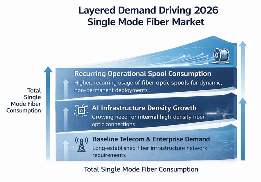
These forces interact rather than operate independently.
When recurring demand expands while upstream capacity remains rigid, price volatility can evolve into structural repricing.
Structural Driver One: Recurring Operational Spool-Based Consumption
A Shift From Installed Assets to Consumable Demand
Traditional telecom fiber deployment installs infrastructure that remains in service for decades. Fiber becomes part of a fixed capital asset base.
By contrast, fiber deployed in specialized long-length spool systems functions differently. In many mission-critical and tethered applications, fiber is deployed dynamically and may not be economically recoverable after use.
This transforms demand from:
- Capital-expenditure driven infrastructure growth to
- Recurring operational inventory consumption
Recurring consumption exerts continuous pull on supply rather than episodic demand spikes.
This distinction is fundamental.
Why Single Mode Fiber Is Central to Spool Systems
Long-length spool-based systems typically require:
- Extended transmission distance
- Low attenuation
- Immunity to electromagnetic interference
- Lightweight construction
Single mode fiber (SMF) uniquely satisfies these criteria.
Multimode fiber lacks comparable transmission range. Copper conductors introduce weight and interference constraints.
As a result, spool-based systems predominantly rely on telecom-grade single mode fiber types such as G652D and bend-insensitive G657 variants.
This ties spool demand directly to the same supply base serving telecom networks and data centers.
Length Profiles and Market Impact
Spool systems may contain several kilometers to dozens of kilometers of fiber per unit.
Even if overall volume remains smaller than global telecom infrastructure demand, the impact can be disproportionate when:
- Demand is recurring
- Deployment cadence is elevated
- Inventory buffers are already thin
- Upstream capacity is slow to adjust
Commodity markets often move at the margin. When available supply tightens, incremental demand layers can shift clearing prices significantly.
Why Recurring Demand Behaves Differently
Infrastructure demand is typically:
- Project-based
- Regionally concentrated
- Time-bound
Operational spool demand can be:
- Recurring
- Less deferrable
- More time-sensitive
- Less predictable
This increases planning uncertainty across the supply chain.
When supply is rigid, time-sensitive demand has greater pricing power.
Structural Driver Two: AI Infrastructure Density Expansion
Operational spool demand does not act alone.
The second major driver of the 2026 surge is AI infrastructure growth.
Optical Density Inside AI Clusters
Modern AI data centers require:
- Massive east-west traffic
- High optical port density
- Low-latency interconnect
- High internal bandwidth
As compute clusters scale, optical links increase non-linearly.
Even if individual cable runs are short, total strand count expands rapidly.
This increases optical density inside facilities rather than expanding geographic network footprint.
Non-Linear Growth Characteristics
AI demand differs from traditional telecom in several ways:
- Globally synchronized investment
- Compressed build cycles
- Rapid scaling waves
- High bandwidth intensity
AI deployments can increase fiber usage without proportional expansion in physical footprint.
This density expansion competes for the same upstream fiber and preform supply.
Layered Demand Effects
When AI density growth overlaps with recurring spool-based operational consumption, demand becomes layered:
- Baseline telecom and enterprise demand
- AI infrastructure scaling
- Operational spool consumption
Layered demand reduces the probability of rapid normalization.
Markets normalize more slowly when multiple demand drivers align in time.
Structural Driver Three: Upstream Preform Constraints
Much discussion focuses on fiber drawing towers.
However, the true structural bottleneck lies upstream — at the preform stage.
The Optical Fiber Production Chain
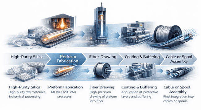
Single mode fiber production includes:
- High-purity silica preparation
- Preform fabrication (MCVD, OVD, VAD processes)
- Fiber drawing
- Coating and buffering
- Cable or spool assembly
Preform manufacturing is capital-intensive and technically demanding.
Drawing towers can be installed faster.
Preform expansion cannot.
Why Expansion Is Slow
Preform capacity expansion requires:
- Capital approval
- Specialized equipment procurement
- Controlled installation
- Process stabilization
- Yield optimization
Typical timelines:
- ~12 months for planning and procurement
- 6–12 months for installation
- Additional time for yield stabilization
Total effective ramp: 18–24 months.
This lag creates structural rigidity in supply response.
Yield and Quality Complexity
Preform production requires:
- Strict dopant concentration control
- Temperature stability
- High purity chemical processes
- Tight quality consistency
Even after new equipment is installed, yield optimization can take several quarters.
This means supply response is never instantaneous.
Capital Discipline After Oversupply
Following prior oversupply cycles, manufacturers have become more cautious in capacity expansion.
Without clear long-term demand visibility, producers may avoid aggressive investment.
Cautious expansion reinforces tightness when demand accelerates unexpectedly.
Historical Context: Why 2026 Differs
2016–2018 Telecom Expansion
- Driven by FTTH rollout
- Regionally concentrated
- Corrected once capacity expanded
- Demand was project-based
Correction occurred within 12–18 months.
2020–2021 Supply Chain Shock
- Driven by logistics disruption
- Temporary in nature
- Normalized once shipping stabilized
This was not structural demand expansion.
2026 Structural Layering
The 2026 surge reflects:
- Recurring operational spool consumption
- AI-driven density scaling
- Globally synchronized investment
- Limited upstream elasticity
Previous cycles were infrastructure-driven or logistics-driven.
This cycle combines recurring consumption with synchronized technology expansion.
That is historically unusual.
Reading Market Signals
To evaluate whether tightness is temporary or structural, observe operational indicators:
Signs of Temporary Tightness
- Quotation validity periods extend
- Lead times stabilize
- Allocation language softens
- Substitution becomes easier
Signs of Structural Tightness
- Quotes remain short-lived
- Lead times vary by grade and region
- Allocation persists despite nominal capacity
- Upstream input constraints dominate planning
Operational signals often provide earlier insight than public commentary.
Scenario Modeling: Three Possible Paths
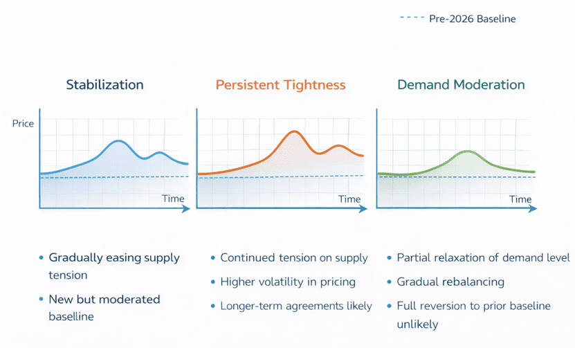
Scenario 1: Gradual Stabilization
Assumptions:
- Operational spool demand stabilizes
- AI growth moderates
- Preform expansion proceeds
Outcome:
- Elevated pricing through 2026
- Softening begins in late 2027
- New baseline above historical lows
Scenario 2: Persistent Tightness
Assumptions:
- Recurring operational demand remains elevated
- AI infrastructure continues expanding
- Upstream expansion remains cautious
Outcome:
- Tight supply through 2027
- Higher volatility
- Greater reliance on long-term agreements
Scenario 3: Demand Moderation
Assumptions:
- Operational demand declines
- AI expansion slows
- Preform expansion exceeds expectations
Outcome:
- Gradual rebalancing
- Partial correction
- Limited probability of full return to prior lows
Even in moderation, structural demand layers may prevent a complete reset.
Structural Implications for Procurement Strategy
If 2026 represents structural repricing:
- Allocation Stability May Outweigh Spot Pricing
Reliability of supply becomes more valuable than marginal cost optimization.
- Long-Term Agreements May Increase
Multi-year agreements may replace short-term spot purchasing.
- Risk Diversification Becomes Strategic
Buyers may diversify sourcing to reduce exposure to single-region bottlenecks.
- Upstream Visibility Gains Importance
Suppliers with integrated or transparent upstream capacity may gain competitive advantage.
Long-Term Market Implications
Commodity markets occasionally undergo structural resets rather than cyclical fluctuations.
If recurring operational spool demand remains embedded alongside AI density growth, the single mode fiber market may transition toward a higher long-term equilibrium band.
Structural repricing does not imply permanent scarcity.
It implies recalibrated baseline expectations.
Markets rarely return fully to prior pricing bands when persistent demand layers remain in place.
FAQ
Why did single mode fiber prices rise so quickly in 2026?
Because multiple demand layers — including recurring operational spool consumption and AI infrastructure expansion — converged while upstream preform capacity remained slow to expand.
Is this mainly a supply problem?
It is a mismatch between layered demand growth and limited short-term supply elasticity at the preform stage.
How long can tight conditions last?
If demand layers persist, tightness can last until upstream capacity expansion is fully ramped and stabilized — often 18–24 months.
Will prices return to pre-2026 levels?
Not necessarily. If structural demand layers remain, the long-term equilibrium may settle above historical lows.
Why is preform production so important?
Preform manufacturing defines upstream capacity limits. Drawing towers can expand more quickly, but preform expansion is slower and more capital-intensive.
How does AI affect fiber demand if cables are short?
AI clusters increase internal optical density and port counts, raising total fiber usage even without geographic expansion.
Final Structural Conclusion
The 2026 single mode fiber price surge cannot be attributed to a single factor.
However, the emergence of recurring operational spool-based consumption introduces a structural demand layer fundamentally different from traditional infrastructure cycles.
When this demand converges with AI-driven optical density expansion and constrained preform elasticity, structural repricing becomes plausible.
The central question is not whether short-term volatility will persist.
The central question is whether 2026 marks the beginning of a new pricing equilibrium in the single mode fiber market.
If recurring operational demand remains embedded in global consumption patterns, this cycle may represent a transition from purely cyclical pricing behavior toward structurally elevated bands.